[TOC]
- Tensorflow supports "half precision" floats -- float16.
- Float32 is called "full precision"/"single precision".
- Float64: "double precision".
- Shuffling = re-sharding = ...
#`8 - Algos.pptx` @ 2/28: **Three Common “Design Patterns” in Big Data Analysis**
##**Caching / memo(r)ization**: process a lot of data that repeats/‘partly overlaps’
- Caches
- In PySpark:
- pyspark's `.cache()`: useful even just for caching a file-loading process.
- Spark gives 5 types of Storage level
- `MEMORY_ONLY`
- `MEMORY_ONLY_SER`
- `MEMORY_AND_DISK`
- `MEMORY_AND_DISK_SER`
- `DISK_ONLY`
> `cache()` will use `MEMORY_ONLY`. If you want to use something else, use `persist(StorageLevel.<*type*>)`.
>
> By default `persist()` will store the data in the JVM heap as unserialized objects. ([source](https://stackoverflow.com/a/43231985/1147061))
- It's a trade-off between:
- IO-efficient and re-useable
- Redundant but parallel
Sometimes you may prefer parallelism more than IO-efficiency!
- the whole **cache** can be considered as a **defaultdict** in Python, defaulting to computing and storing the executionPlan.
- But it's more than just naive key-lookups -- consider `A join B` and `B join A`: **DFs are in different order but should yield identical results.** There should be a "key interpreter/canonicalizer" that is aware of this (perhaps by a "sort tuple" procedure, as seen in page 11).
- There's a **limit** (e.g. capacity of your memory) to caches, so:
- Manually, you should:
- only cache things you gonna **reuse**
- remember to `unpersist` when you are done with it
- be aware of constantly updating data source -- validity of cached DFs may **expire** and thus should be dropped.
- if by manual selection the cached data is still exceeding the memory's capacity, the computing platform may intervene and prioritize cached items:
- either by dropping Least Frequently Used (LFU) items
- or dropping Least Recently Used (LRU) items.
_(code demonstrated on page 13, using another dictionary to store last access time)_
- Difference between caching and memoizing: ([source](https://stackoverflow.com/a/6469677/1147061))
- "memoization" is "caching the result of a **deterministic** function" that can be reproduced at any time given the same function and inputs.
- "Caching" includes basically **any output-buffering** strategy, whether or not the source value is reproducible at a given time. In fact, caching is also used to refer to *input* buffering strategies, such as the write-cache on a disk or memory. So it is a **much more general** term.
- memoization
- a key concept in **dynamic programming**
##process many different tasks in ‘parallel’ (3/12/2018)
- **Task scheduling** (Multitasking/task switching)
- key concepts: ([source](http://masnun.rocks/2016/10/06/async-python-the-different-forms-of-concurrency/))
- **Sync:** Blocking operations.
- **Async:** Non blocking operations.
- **Concurrency:** Making progress together.
- **Parallelism:** Making progress in parallel. *Parallelism $\in$ Concurrency.*
- Concurrency in Python
- **Manual** approach: `data=operator(data)` approach - using `queue`
- **Automatic** approach (Great reading: [source](http://masnun.rocks/2016/10/06/async-python-the-different-forms-of-concurrency/))
- `multiprocessing` populates multiple processes
- `threading` uses threads
- `concurrent.futures` is a simpler interface to those two above
- `asyncio`
- **Random exploration via genetic algorithms**
- randomness + parallelism
- consider it a non-exhausive search -- by using random sampling.
- also this makes it a good candidate to make approximate algorithms
##**Search and constraint solvers**: find an item, a parameter, etc. that maximizes an objective”
- Planning consists of:
1. Defining start and goal states
2. Defining a sequence of actions and constraints about how they can be used
3. Defining a search strategy
4. Finding pruning methods
- pruning
- forward chaining
- **backward chaining** -- allows for more advanced pruning, such as "branch-and-bound pruning"
# @3/14/2018 - **Unsupervised data analysis**
## Principal Component Analysis (PCA) -- Group similar features together (roughly)
- PCA can be viewed as: A rotation to a new coordinate system (a.k.a. "a projection to **a new space**") to **maximize the variance** in the new coordinates.
- PCA is scale-variant -- rescaling data w.r.t. any feature will change PCA result. Also, center ("mean") of data should really be at origin.
- Thus, **standardization** is important.
- but be aware of log-scaled raw features!
- Realized by computing the covariance matrix.
- Its eigenvectors are our principal components (from original space to PCA-ed space).
- To compute for them: use single value decomposition (SVD) with fast algorithms like "randomized SVD".
- Its eigenvalues are the covariance explained. Use eigenvectors in descending order of this!
- Excessive principal compoenents are merely capturing noise in the data.
- compare with: t-distributed Stochastic Neighbor Embedding (t-SNE)
- non-deterministic (each run of t-SNE, even on the same set of data, can give different results)
- Local-focused
- coordinates mean nothing. Information is all in proximity.
- which leads to the topic of clustering...
##Clustering -- Group similar items together
- K-Means
- Minimizes within-cluster Sum of Squared Errors (SSE) (a.k.a. distortion function).
- Non-convex.
- K-means++: Initializes centroids as far away from each other as possible.
- K-means in SQL (see `.sql` file)
- pyspark.mllib.clustering has k-means packaged: KMeans, KMeansModel.
- Elbow method for choosing the right number of clusters
- alternative to centroid is the "medoid": while centroid is the numerical average for continuous values, themedoid is for categorical features -- choosing the most representative/frequent point.
- hierichical clustering
- major difference with k-means: # of clusters is determined iteratively, rather than specified upfront.
- two approaches:
- agglomeative (a.k.a. AHC or HAC): start with single-item clusters and keep merging closest items. <- we will focus on this
- Divisive: start with one cluster containing all datapoints. keep dividing till all clusters are single-points.
- distance between clusters
- **single** linkage:
- compute distance between the most **similar** members for each pair of clusters.
- AHC: Merge the clusters with the **smallest** distance.
- **Complete** linkage:
- Compute distance between the most **different** members for each pair of clusters.
- AHC: Merge the clusters with the **smallest** distance.
- implementation in spark
- spark.mllib contains divisive, not agglomeative
- UBer has their own implementation of AHC
- pros and cons
- Pros:
- plots dendrograms -- helps taxonomy
- can stop at any number of clusters at will
- Cons:
- Does not scale well
- (K-means too) assumes clusters have **spherical shape**
- Density-Based Spatial Clustering of Applications with Noise (DBSCAN)
- each point is assigned to one label: (great read: [source](https://www.cse.buffalo.edu/~jing/cse601/fa12/materials/clustering_density.pdf))
- A **point** is a core **point** if it has more than a specified number of **points** (MinPts) within Eps—These are **points** that are at the interior of a **cluster**.
- A **border point** has fewer than MinPts within Eps, but is in the neighborhood of a core **point**.
- A noise **point** is any **point** that is not a core **point** nor a **border point**.
- **Handles non-spherically-clustered datasets**!
- Noise tolerant.
###How to they compare - time complexity:
(n: # of points; d: # of dimensions; k: # of clusters.)
- k-means: `d * n * k * # of iterations * # of restarts`
- Agglomerative: `>dn^2`
- DBSCAN: depends on thregion size; suffers from thecurse of dimensionality
### Other Techniques
- Locally sensitive hashing: ...
- MinHash: Hashing for Jaccard Distance
# Supervised Learning
## @03/26/2018 - decision trees
- types of supervised learning
- **classification**: y is categorical
- **Regression**: y is continuous
- Model may be:
- Parametric: a known funcgional form -- we are here to estimate values
- Linear and logistic regression
- Non-parametric: no functional formv assumed
- decision tres and random forests
- boosted models
- semi-parametric: so many parameters as to be effectively non-parametric
- e.g. neural networks
- Decision trees
- can be used for feature selection
- splits first on the option that provides the highest Information Gain
- The more uniformly distributed the data is, the lower a Gini Index it has, the higher an Entropy it has.
- very susceptible to overfitting
- if features are highly correlated, use PCA first
- balance training data amount for each label
- limit maximum depth
- keep minimum number of samples for a split from being too low
- prune after training
- Ensemble version: random forest
- bootstrap -- sample (with replacement) for each member (individual decision trees).
- majority vote (or average) members' outputs.
- Variation: extremely random forests
- Not only training data is randomly sampled,
> instead of looking for the most discriminative thresholds, thresholds are drawn at random for each candidate feature and the **best of these randomly-generated thresholds** is picked as the splitting rule. ([source](http://scikit-learn.org/stable/modules/ensemble.html))
- d-tree can tell repetitive features and mark them "less important".
- summary
- decision trees
- Fast to train
- easily interpretable
- random forests
- highly accurate
- does not require hyperparameter search
- both
- scale **invariant** -- these models are non-parametric!
- handles both numerical and categorical data
## @03/28/2018 - regression, boosting and SVMs
### Regression
- **Parametric or not?** Linear regression models, and therefore logisitic regression too, are examples of parametric models.
- **A Word On Regularization**: No matter L2 regularization ("ridge"), L1 regression ("lasso") or PCR, they all decides for each feature how much it should be suppressed before fed into a linear regression model.
####The Linear Regresion Family
- Linear Regression
- minimizes root mean squared error (RMSE)
- in practice, the `sqrt()` is omitted - minimizes "MSE".
- brightside: it has a closed-form solution, but there's potential problem:
- space complexity: $X^T\cdot X$ can be big -- $n^2$. May not fit in memory.
- time complexity: $n\cdot d^2$ (d is the # of features) -- can be big.
- If d>n, then the X-inversion step will hit a singular point error and fail.
- Scale invariant -- needs no normalization
- **ridge regression** := Linear regression + $\lambda w^T\cdot w$
- Minimizes MSE + L2 penalty
- a.k.a. "ridge", "L2 regularization", etc.
- idea: shrinks all the weights a little -- just shrink, not making any feature's weight go to zero.
- NOT LONGER scale invariant
- **Elastic net** := linear regression + $\lambda_1 w^T\cdot w$ + $\lambda_2$ L1 penalty
- L1 penalty is also called the "lasso".
- Idea: L1 can drive least-important features' weights to zero.
- now you have two hyperparameters for regulation: $\lambda_1$ and $\lambda_2$
#### Principal Component Regression
1. Do PCA on X.
2. Project X onto the PCXA loadings: $T=X\cdot W$ (nxk = nxp * pxk)
3. Use T as training data instead of X. Usually linear regression too.
4. To predict using this PCR model, project test examples to W, then feed into the "linear regression" sub-model.
- Often used in computational linguistics.
- Different from the ones introduced above: PCR can be called a "semi-supervised learning algorithm"
- PCA part is unsupervised
- actual regression part is supervised.
- just like PCA -- not scale-invariant
####Logistic Regression := linear regression + filtering using logistic function + binarizing results to 0&1
- for binary labels (thus for classfication, rather than prediction)
- Since the output will be binarized to 0&1, the value before this binarization is considered to be the probability -- probability estimate: $\sigma(w^T\cdot X)$
### Boosting
- train a series of dumb classifiers, each one focusing more on the examples mis-classified by the previous one.
- is an ensemble method
### SVM
- also for classification.
- maximizing margin...
- "Soft margin": we can trade-off between margin width and violations of the border.
- Usually uses "hinge loss" -- don't care about correctly-classified examples.
- kernels - feature engineering (not covered)
- linear
- polynomial (order can be configured)
- radial basis (a.k.a. gaussian)
- when use a kernel, not scale-invariant.
## @04/02/2018: Tuning and evaluating classifiers
- Complexity - we want to find the optimal complexity that balances the training error and test error -- avoid underfitting and overfitting.
- visualize with learning curves.
- k-fold cross validation
- Holdout sets: part of training data held out and used like a test set.
- some curves:
- validation curve: x-axis is the value of hyper-parameter; y-axis is the score. 
- take the peak.
- learning curve: x-axis is the percentage. 
- Validation/test score should be also high. Don't let it drop -- it would be overfitting.
- ROC curves:
- 
- confusion matrix and all of those performace metrics. (probably omittable)
- accuracy is often the wrong measure.
- some are: error, precision, recall, F1 score.
## @4/4/2018 - Artificial Neural Networks
- gradient descent
- analytical or numerical derivative
- variations in terms of training data granuity:
- **(vanilla) gradient descent** requires all training data to be loaded to compute the gradient.
- **stochastic gradient descent** calculates the gradient on a per-example basis, allowing for online-learning.
- **Mini-batch**: updates the model every $k$ observations -- a hybrid approach to the two above.
- Can get caught in **local minima** -- alternative, **simulated annealing**, uses randomness.
- according to a "cooling schedule", is initially more likely to randomly jump.
- still no gurantee, but lready less susceptable to local minima.
- logistic regression is actually a basic "artificial neuron"
- activation function
- uses sigmoid function as "model" -- in this sense, it's similar to logisitic regression.
- Alternative to sigmoid function if you want a **hard classifier**: heaviside function.
- A neuron can take multiple inputs -- just like thsoe features inputed in logisitic regression.
- with an extra "always-on" (i.e. always emitting $1$) input, called "bias". Its effect to the neuron's decision is controlled by its associated weight instead of its value itself.
- regularization is NOT applied on it.
- $\eta$ is the learning rate.
- A perceptron is a single layer of many such neurons.
- consider this as multiple regressions running at once (each neuron being one).
- still learns a linear boundary -- gurantees conergence if only the training data is linearly seperable.
- to deal with non-linearly-separable data,
- SVM uses kernels
- neural nets use extra layers. See below.
- (doesn't mean that technically we cannot use kernels with perceptrons)
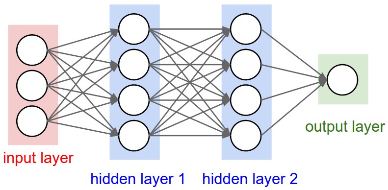
- deeper networks are just models of multiple layers as such -- feed-forward networks
- can deal with non-linearly-separable data.
- **structure:** Input layer -> hidden layer(s) -> output layer
- each layer can have multiple neurons.
- activation function: usually ReLU ("rectified linear") here.
### @4/9/2018 - Convolutional Neural Networks
Great reading: [source](http://cs231n.github.io/convolutional-networks/).
- for images
- ==CNN uses local receptive field==
- types of layers
- **Convolution** connects the *receptive field* to a neuron in the next layer
- often with overlap (“strides”). "Stripe" is the steplength.
- Will hit border of image -- needs zero-padding (how much? also a hyperparam)
- kernels in CNN are called "filters".
- > The spatial extent of this connectivity is a hyperparameter called the *receptive field* of the neuron (equivalently this is the filter size).
- **Pooling** does aggregation (often: max)
- pooling ("downsampling"): most often max-pooling, etc.
- **Detection** uses sigmoid or RLU
- usually uses ReLU as activation function -- Cheaper to calc deriv
- ==back propagation==.
- ==ways of regularization==:
- L2
- Max norm (L∞)
- Early stopping
- ==Dropout==: randomly dropping out connections between layers (?).
- techniques about **Gradient descent**
- Gradient descent
- - stochastic
- gradient clipping
- ==Minibatch==
- Momentum
- Learning rate adaptation
- learning rate adaption:
- Adagrad: make the learning rate depend previous changes in *each* weight
- **Semi-supervised learning**
#@04/11/2018 - Time Series
- What makes a TS different from say a regular regression problem?
1. It is **time dependent**. So the basic assumption of a linear regression model that the observations are independent doesn’t hold in this case.
2. Along with an increasing or decreasing trend, most TS have some form of **seasonality trends**, i.e. variations specific to a particular time frame. For example, if you see the sales of a woolen jacket over time, you will invariably find higher sales in winter seasons.
- some techniques
- use a moving average to smooth out short-term fluctuations and highlight longer-term trends or cycles.
- use `log()` if data appears to be exponential -- this can give something showing more linearity -- easier to deal with.
- Time series are **stationary** if they do not have trend or seasonal effects.
- Summary statistics (such as the mean or variance) calculated over stationary time series are consistent over time.
- Stationarity is an assumption underlying many statistical procedures used in time series analyses, so non-stationary data is often transformed to become stationary. **How to make a time series stationary**:
- **Estimate and eliminate trend**
- - **Transformation** – e.g. take log, which penalizes higher values more than smaller ones.
- **Aggregation** – take average for a time period like monthly/weekly averages
- **Smoothing** – take rolling (moving) averages.
- - “weighted moving average” gives more recent values a higher weight than older values
- In an “**exponentially weighted moving average**”, weights are assigned to all the previous values with a decay factor.
- No data is left beind -- all taken in to consideration.
- **Polynomial fitting** – fit a regression model
- **Remove trend and seasonality**
- - **Differencing** – taking the difference with a particular time lag
- **Decomposition** – modeling both trend and seasonality and removing them from the model.
- Converting a time series from one frequency to another
- Downsampling – higher to lower frequency
- Upsampling – lower to higher
- **Statistical test: Augmented Dickey-Fuller (ADF)**
- Tests the **null hypothesis** that the time-series is non-stationary.
- The more negative the Test Statistic is, the stronger the rejection of the hypothesis.
- how to make predictions with time series data
- Models
- **Auto-Regressive model AR(p)**
- x(t) = c0 + ct-1 x(t-1) + ct-2 x(t-2) +….+ ct-p x(t-p) + É√t
- **Moving Average model (MA(q))**
- x(t) = c0 + c t-1 e(t-1) + c t-2 e(t-2) +….+ c t-q e(t-q) + É√t
- e(t) = É√t = error in prediction at time t
- **Auto-Regressive Integrated Moving Averages (ARIMA)** forecasting
- linear equation based three parameters, (p, d, q)
- **p auto-regressive (AR) terms** (a.k.a. "lags of dependent variable"). For instance if p is 5, the predictors for x(t) will be x(t-1)….x(t-5).
- **q moving average terms (MA)** (a.k.a. "lagged forecast errors in prediction equation"). For instance if q is 5, the predictors for x(t) will be e(t-1)….e(t-5) where e(i) is the difference between the moving average at ith time and actual value.
- **d non-seasonal differences**
- - **How to determine p and q?**
- Plot autocorrelation functions and partial autocorrelation functions and see when they cross an upper confidence interval.
- For this data, p=q=2.
- technique: **Differencing**
- - y(t) = x(t) – x(t-1), Then fit the model on y(t)
- Makes the process more stationary
# @04/16/2018 - TensorFlow
- TensorFlow is based on a **Computation Graph** executed in parallel.
- All data are represented as tensors -- analogy to columns.
- Two sets of APIs:
- one resembles sklearn
- to initialize a classifier, you have to specify feature columns -- different from sklearn.
-
- one lower level
- TensorFlow column datatypes (`tf.contrib.layers.[...]`)
- for real-valued features: `real_valued_column`
- for categorical features:
- If you know all possible values: use `sparse_column_with_keys`.
- If you cannot iterate over all categories (or simply want to allocate ordinal values to categorical values on the fly): use `[...]_hash_bucket`.
- choose bucket amount wisely -- balance between hashing collisions and memory consumption
- use numerical feature as categorical: `bucketized_column`
- For feature combinations: `CrossedColumns`
## Distributed TensorFlow
- Master nodes know the whole Computation Graph.
- Worker nodes know only the operation it's assigned with.
- worker 0 may be the "parameter server" and hold mutable data (weights, biases, etc.)
- worker 1 may hold the training data and compute some operations.
- Data can be stored on a Spark cluster (i.e. in HDFS) and **streamed** to the TensorFlow cluster. Yahoo did this: `TensorFlowOnSpark`.
## Recurrent Neural Networks (RNN) - Handles Time Series
- two approaches to time series
- use a standard neural net or CNN
- such as a nonlinear AR(k) model
- use a RNN
- generalize HMMs or Linear Dynamical Systems
- only choice if inputs are of varying lengths
- See **standard hidden markov model**: each "stage" takes the previous result as part of input.
- variations
- Long Short Term Memory (LSTM)
- gated RNNs
- stacked RNNs
- can be used...
- ... to predict the next observation given past observations (like an ARIMA model)
- ... to map one sequence to another sequence ("encoder-decoder" structure)
- translates sentences from one language to another
- chatbot
- auto-caption image
# @04/18/2018 - Online Learning
- Online learning methods
- Least mean squares (LMS)
-
Online regression -- L2 error
- Perceptron
- Idea
- if we get it right: no change;
- if we got it wrong: $\vec w_{i+1} = \vec w_i + \vec y_i \vec x_i$.
- This makes $w$ look more like $\vec x_i$, thus the hyperplane defined by $\vec w$ is more orthogonal to this example of $\vec{x}_i$.
- In practice, we use **averaged perceptrons** -- a cheap approximation to **voted perceptons**.
- Return as its final model the average of all intermediate models
- sounds like a ensemble learning, but actually it just keeps one single, averaged model at any time.
- Better than voted perceptons: run-time nearly as fast as single percepton.
- can use **kernels**.
-
variation: Online SVM -- Hinge loss
-
Online K-means
- different from Neural nets: we look at each example and throw it away.
## Analyzing Real-Time Data Streams
- **Data Streams**
- may not be peroidic
- update most often have a delay from actual event
- timestamp reported may...
- not be precise (time sync server problem, etc.)
- has timezone problem (sometimes needed, sometimes to remove)
- consider operations on data streams to be "continuous queries".
- outputs can also be considered data streams
- types
- cumulative operations -- performed on all data streamed
- **Rolling or windowed** operations (e.g. a "last-two-minute window".)
- tumbling windows: no overlap
- sliding windows: move a fixed length every step (like a queue)
- sliding + partitions windows: shards data according to key to two sliding windows
- architechture
- lambda architechture
- Apache Spark Streaming
- ...
# @04/23/2018 - Stream Processing Systems
(a wrap-up of streaming processing)
- Apache Spark
- component:
- data streams exposed as ever-changing **dataframes**
- We define **windows** over streams
- "joins/merges" make sense on windows, not much on streams themselves.
- Based on “micro batching” – periodic invocations of Spark Engine on batches
of tuples
- To process:
- `StreamingContext` gets started
- `awaitTermination()` is run
- Can process whatever is in the DataStream as a DataFrame
- Can run `countByWindow()` etc. to get time-based or tuple-based windows
- Apache Storm (and Heron): distributed streams among distributed modules
- components
- **spout**: interfaces with the world, **produce** streams
- emits lists of tuples
- **bolt**: receive streams, optionally producing streams + read/update states.
- structure: spouts and bolts are usually pipelined. They can also be **stacked** (for distributed computing).
- promises robust execution (even when compared to Spark)
- can be used to mimic MapReduce structure,
- To Storm, `streamparse` is what `pyspark` is to Spark.
# Visualization
- Get a **holistic** sense of **data** as we load + analyze it
- histograms, scatter plots, correlations, time series
- Understand our **algorithms’ performance**
- learning curve, validation curve, ROC graph
- Present information as part of a **report** or “**dashboard**”
- figures illustrating performance (in the economic sense, etc.)
- Potential Kinds of Plots
- Exploratory graphics – for the data scientist. Want to create rapidly, iterate,
- Communication graphics – for you to communicate your findings, Again, iteration is important
- “Grammar of Graphics”
- Basis of R’s ggplot2
- Python port: `ggplot`
- Divides plots into:
- layers
- data
- aesthetic mappings
- geometric objects
- **statistical transformations**
- position adjustments
- scales
- coordinate system
- facets (groups)
- more advanced visualization in python
- `seaborn`: Builds upon `matplotlib` with a focus on statistical plots
- `lightning` + `d3.js`: “Dashboards”
- requires server -- Jupyter is also a web server
# @04/25/2018 - Data Science Ethnics
- Why do people do the right thing?
- Morality (Ethnics)
- Enthical principles
- **Autonomy**: The right to control your data, possibly via *surrogates*
- **Informed Consent**: You should explicitly approve use of your data based on understanding
- required in human-subjects research
- must understand what is being done
- must voluntarily consent to the experiment
- must have the right to withdraw consent at any time
- but no one requires them in “ordinary conduct of business”
- consequently we are constantly subject to tests such as A/B tests.
- **Beneficence**: People using your data should do it for your benefit
- or at least **Non-maleficence**: Do no harm
- **Differential privacy** aims to maximize the accuracy of queries from statistical databases while minimizing the chances of identifying its records.
- we want results that are ...
- reproducible
- fair